-
PDF
- Split View
-
Views
-
Cite
Cite
Joseph D. Manthey, Luke C. Campillo, Kevin J. Burns, Robert G. Moyle, Comparison of Target-Capture and Restriction-Site Associated DNA Sequencing for Phylogenomics: A Test in Cardinalid Tanagers (Aves, Genus: Piranga), Systematic Biology, Volume 65, Issue 4, July 2016, Pages 640–650, https://doi.org/10.1093/sysbio/syw005
Close - Share Icon Share
Abstract
Restriction-site associated DNA sequencing (RAD-seq) and target capture of specific genomic regions, such as ultraconserved elements (UCEs), are emerging as two of the most popular methods for phylogenomics using reduced-representation genomic data sets. These two methods were designed to target different evolutionary timescales: RAD-seq was designed for population-genomic level questions and UCEs for deeper phylogenetics. The utility of both data sets to infer phylogenies across a variety of taxonomic levels has not been adequately compared within the same taxonomic system. Additionally, the effects of uninformative gene trees on species tree analyses (for target capture data) have not been explored. Here, we utilize RAD-seq and UCE data to infer a phylogeny of the bird genus Piranga. The group has a range of divergence dates (0.5–6 myr), contains 11 recognized species, and lacks a resolved phylogeny. We compared two species tree methods for the RAD-seq data and six species tree methods for the UCE data. Additionally, in the UCE data, we analyzed a complete matrix as well as data sets with only highly informative loci. A complete matrix of 189 UCE loci with 10 or more parsimony informative (PI) sites, and an approximately 80% complete matrix of 1128 PI single-nucleotide polymorphisms (SNPs) (from RAD-seq) yield the same fully resolved phylogeny of Piranga. We inferred non-monophyletic relationships of Pirangalutea individuals, with all other a priori species identified as monophyletic. Finally, we found that species tree analyses that included predominantly uninformative gene trees provided strong support for different topologies, with consistent phylogenetic results when limiting species tree analyses to highly informative loci or only using less informative loci with concatenation or methods meant for SNPs alone.
Restriction-site associated DNA sequencing (RAD-seq; Miller et al. 2007) and target capture of specific genomic regions, such as ultraconserved elements (UCEs; Faircloth et al. 2012), are emerging as two of the most useful methods for phylogenomics. RAD-seq was initially developed for identifying and studying recent population divergences, and has been successfully utilized for phylogeographic studies in a variety of organisms, including Sarracenia pitcher plants (Zellmer et al. 2012), Lycaeides butterflies (Gompert et al. 2010), and an assortment of bird species (McCormack et al. 2012). At deep timescales, RAD-seq may recover few orthologous loci among divergent lineages, with potential rate bias in the loci that do overlap (i.e., they are identified as orthologous because of slow mutation rate; Rubin et al. 2012). Conversely, target-capture using UCEs was developed for studying deep divergences and difficult phylogenetic questions, and has since been utilized to infer higher-level phylogenies in a diverse set of taxa, including Hymenoptera (Faircloth et al. 2014), ray-finned fishes (Faircloth et al. 2013), and birds (McCormack et al. 2012). In contrast to RAD-seq, the drawbacks of using UCEs are at recent timescales, due to insufficient time to accumulate informative sites next to the conserved target regions (e.g., Smith et al. 2013).
Although many studies have investigated systematic or phylogeographic questions using one of these methods, few have explored both methods in the same study system. Harvey and colleagues (2013) used UCEs and RAD-seq to study phylogeographic patterns in a widespread Neotropical songbird (Xenops minutus) with shallow divergences (<5 myr); they identified concordant phylogenetic relationships between data sets. Conversely, Leaché and colleagues (2015) used sequence capture and RAD-seq to study deep systematics (15–55 myr) of phrynosomatid lizards; here, the authors found different results between data sets depending on which pipeline and filtering steps were used.
In addition to the inherent differences between target-capture and RAD-seq data sets, other issues may influence species tree inference within target-capture data sets alone. Multiple simulation studies have identified that species tree inference is negatively influenced by inclusion of weak—or largely uninformative—loci (Lanier et al. 2014; Liu et al. 2015). With the rapid expansion of target-capture data for phylogenetic inference, it is necessary to assess the impacts of uninformative loci (and their estimated gene trees) on species tree inference across methodologies with empirical data sets. In contrast, because RAD-seq loci are inherently short—often less than 100 bp—phylogeneticists have generally not attempted species tree reconstruction using the underlying gene trees. Therefore, we are limiting our assessment of low information loci on species tree inference to target capture, as we already presume that gene trees generated from RAD loci will be mostly unresolved.
Here, we extend previous comparisons of sequence capture and RAD-seq for phylogenetics in a genus of songbirds (Piranga, Aves: Cardinalidae) with a range of divergence dates [0.5–6 myr based on mitochondrial DNA (mtDNA); Burns 1998] among 11 recognized species and recognized intraspecific divergences within three of the species (Table 1; Burns 1998, IOC World Bird List v5.1). With most of the intragenus relationships unresolved from mtDNA alone (Burns 1998, Shepherd and Burns 2007), Piranga provide an empirical system that is an appropriate size and age to examine the relative utility of phylogenetic inference using RAD-seq- and UCE-based data sets.
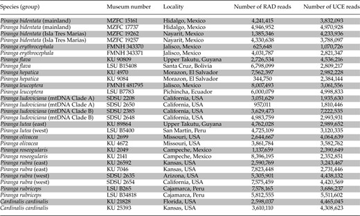
Samples used in this study, their museum voucher numbers, locality to state and country, number of RAD-seq single-end reads, and number of UCE paired-end reads (read 1, read 2, and singletons), both following quality control
 |
 |
Notes: KU, University of Kansas Natural History Museum; LSU, Louisiana Museum of Natural Science; FMNH, Field Museum of Natural History; SDSU, San Diego State University Museum of Biodiversity; MZFC, Museo de Zoología de la Facultad de Ciencias at Universidad Nacional Autónoma de México.
Samples used in this study, their museum voucher numbers, locality to state and country, number of RAD-seq single-end reads, and number of UCE paired-end reads (read 1, read 2, and singletons), both following quality control
 |
 |
Notes: KU, University of Kansas Natural History Museum; LSU, Louisiana Museum of Natural Science; FMNH, Field Museum of Natural History; SDSU, San Diego State University Museum of Biodiversity; MZFC, Museo de Zoología de la Facultad de Ciencias at Universidad Nacional Autónoma de México.
We used Illumina sequencing to obtain RAD-seq and UCE data sets for 28 individuals across 11 species in Piranga (Table 1). With these data, we used seven species tree estimation methods to investigate the following questions: 1) Do RAD-seq and UCE data sets perform similarly—that is, provide sufficient phylogenetic signal—across a range of timescales (0.5–6 myr) common in many phylogenetic studies? 2) Do species tree analyses of RAD-seq and UCE data sets estimate comparable species relationships? 3) How do UCE loci with few or no informative sites influence species tree estimation?
Methods
Sampling and Sample Preparation
Fresh tissue or blood samples of 28 Piranga individuals, two each per recognized species-level taxonomic unit (Burns 1998, IOC World Bird List v5.1) as well as each genetically distinct lineage (e.g., Shepherd and Burns 2007), were obtained from natural history museums (Table 1). Two samples of Cardinalis cardinalis were used as outgroup individuals (Klicka et al. 2007). Multiple intraspecific lineages were included in analysis for Piranga bidentata, Piranga ludoviciana, and Piranga rubra (Table 1), for which multiple clades have been identified or hypothesized. We used a QIAGEN DNeasy blood and tissue kit to extract genomic DNA from each individual. We used Qubit Fluorometric Quantitation (Life Technologies) to quantify and standardize DNA concentrations of all samples.
Sequence Capture Laboratory Procedures and Bioinformatics
We performed target-capture with the Tetrapods-UCE-5Kv1 probe set (available at ultraconserved.org), which targets 5060 UCE loci. Initially, genomic DNA (∼500 ng) was fragmented using a Covaris S220 focused-ultrasonicator (175 W peak incident power, 2% duty factor, and 200 cycles per burst for 45 s). Sonicator conditions were based on optimized settings for unrelated UCE projects at KU using other avian samples. We then prepared sequencing libraries from the fragmented DNA using Kapa Biosystems Library Prep Kits (KBLPK; Kit: KK8201). Samples were subject to end repair and A-tailing following KBLPK instructions. We ligated adapters compatible with the iTruStub dual indexing system (available at baddna.org). Samples were subjected to limited-cycle (10 cycles) PCR to index and amplify individual samples prior to UCE enrichment, followed by pooling of indexed samples (16 samples per pooled library, including two samples from an unrelated project). We enriched the pooled libraries for the 5Kv1 probe set using a Mycroarray MyBaits Kit, followed by a brief (16–17 cycles) PCR reaction to amplify the small amount of each library enriched for UCEs. Although the protocol recommended 12–16 cycles at this step, we ran 17 cycles of PCR on one library to compensate for a lower yield in the UCE enrichment step. The pooled libraries were tested for quality and quantity of DNA using quantitative PCR and the Agilent Tapestation at the University of Kansas Genome Sequencing Core Facility, followed by sequencing of 100 bp paired-end reads on a partial (31.25%) lane of an Illumina HiSeq2500.
Bioinformatics of UCE data largely used the PHYLUCE software package of Python v2.7 scripts (Faircloth 2015). The illumiprocessor.py script was used to trim adapter contamination and check quality of sequencing reads. Next, we used Trinity (version: rnaseq_r2013_08_14; Grabherr et al. 2011) to assemble contigs for each individual. We matched our assembled contigs to the UCE probe set using the match_contigs_to_probes.py script. We aligned each UCE locus using the seqcap_align_2.py script, which batch calls the use of MAFFT (Katoh and Standley 2013). Finally, custom R (R Development Core Team 2012) and Python scripts were used to obtain summary statistics of all loci and convert file types for various phylogenetic analyses (see Data Accessibility and Supplementary Information, available on Dryad at http://dx.doi.org/10.5061/dryad.j5n06).
RAD-seq Laboratory Procedures and Bioinformatics
We performed a single digest modified RAD-seq (Miller et al. 2007; Andolfatto et al. 2011) protocol to obtain many anonymous genetic loci. Genomic DNA samples (∼50 ng per sample) were initially digested with the restriction enzyme NdeI as a first step to produce a reduced representation genomic library. We used NdeI because of positive results from previous projects (e.g., Manthey and Moyle 2015) and the required overhang for the associated indexing barcodes (Andolfatto et al. 2011). We ligated custom adapters with attached barcodes for multiplexing, followed by pooling of samples. Each sample was barcoded in triplicate (Supplementary Table S1, available on Dryad) to minimize sample bias from individual barcodes. We used a Pippin Prep electrophoresis cassette (Sage Science) to size select fragments in the range of 450–600 bp. Following size selection, samples were subjected to a brief polymerase chain reaction (PCR) of the pooled samples in duplicate, which added standard Illumina sequencing indices (i.e., additional indices to dual-index; Andolfatto et al. 2011). The pooled libraries were tested for quality and quantity of DNA using quantitative PCR and the Agilent Tapestation at the University of Kansas Genome Sequencing Core Facility, followed by sequencing of 100 bp single-end reads on a single lane of an Illumina HiSeq2500.
We used the STACKS (Catchen et al. 2011) pipeline to assemble loci de novo from the fastQ files obtained from the Illumina sequencing run. We assigned sequence reads to individuals and removed reads of poor quality using the process_RADtags script included in the STACKS pipeline. For inclusion, sequencing reads were required to have an average phred score of 10 in sliding windows of 15 bp. We removed sequences lacking the restriction site or containing possible adaptor contamination. Next, we used the ustacks, cstacks, and sstacks modules of STACKS with the default settings, with the exception of allowing up to five mismatches between individuals (94% sequence identity between individuals' stacks). The mismatches setting was changed to increase the number of loci recovered across individuals, as the default value of 2 would have required a 98% sequence identity across each RAD locus. Finally, we created a SNP data set using the populations module of STACKS with the following restrictions: minimum stack depth of five, a minimum of one individual per lineage [as informed from a RAxML (Stamatakis 2014) tree produced from concatenated UCE data (Table 1; Fig. 1)], minor allele frequency of 0.05, and observed heterozygosity across all individuals no greater than 0.5 (to reduce inclusion of paralogous loci). To assess the effect of stack depth, we reran the populations module with varying minimum stack depths (, 10, 15); here, the number of loci changed among data sets, while pairwise comparisons of genetic differentiation ( remained the same () and phylogenetic relationships did not change (Supplementary Information, available on Dryad) with the exception of the Hepatic Tanager clade (see “Results” section).
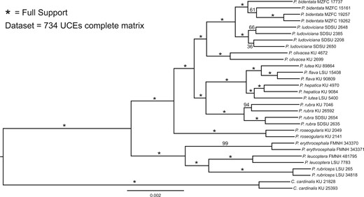
Maximum-likelihood phylogeny of the complete concatenated UCE data set. Support values are based on 1000 quick bootstrap replicates.
Phylogenetic Inference Using UCEs
We used two phylogenetic methods with the concatenated complete matrix (all individuals sampled; 734 loci) data set. First, we used maximum likelihood in RAxML v8.1.18 (Stamatakis 2014) with a GTR+G model of sequence evolution. Support was assessed using 1000 rapid bootstrap replicates. Second, we estimated a species tree using SVDquartets (Chifman and Kubatko 2014) implemented in PAUP* v4a142 (Swofford 2003). SVDquartets samples quartets of individuals' sequences and infers an unrooted phylogeny, followed by species tree inference using all sampled quartets. With this method, we exhaustively sampled quartets from the data set and inferred a species tree from the quartets.
In addition to analyses utilizing concatenated data sets, we inferred species trees using four methods that sample individual gene trees to infer a species tree. For these species tree analyses, we used three data sets: 1) the complete data matrix (all individuals sampled; 734 loci), 2) all loci in the complete data matrix with 10 or more parsimony informative sites (PIS; 189 loci), and 3) all loci in the complete data matrix with 20 or more PIS (70 loci). This allowed us to assess the impact of uninformative gene trees on species tree reconstruction methods, as uninformative loci have been shown to influence summary-based species tree methods (Lanier et al. 2014; Liu et al. 2015).
To estimate gene trees for each locus, we used the Cloudforest pipeline (available at github.com/ngcrawford/CloudForest), which implements MrAIC to estimate the best substitution model for each locus, and then uses PhyML (Guindon et al. 2010) to estimate gene trees. For each data set, 100 multilocus bootstraps (Seo 2008) were performed; each bootstrap resamples loci within the data set, as well as bases within each locus. Because this process resamples loci across the entire data set, the bootstrapping procedure was performed separately for each data set (based on PIS; see Data Accessibility and Supplementary Information, available on Dryad). To ensure that species trees estimated from PhyML gene trees were robust, we also created multilocus bootstrapped gene tree data sets using RAxML (GTR+Gamma model of sequence evolution). Again, as for the PhyML gene trees, each locus analyzed with RAxML was subject to multilocus bootstrapping.
Using the gene trees as input, we used three methods of species tree inference: 1) Species trees from average ranks of coalescence (STAR; Liu et al. 2009), 2) accurate species tree algorithm (ASTRAL; Mirarab et al. 2014), and 3) maximum pseudo-likelihood of estimating species trees (MP-EST; Liu et al. 2010) These three species tree methods were performed for both PhyML and RAxML generated sets of gene trees.
We also used Bayesian Evolutionary Analysis by Sampling Trees [*BEAST (Heled and Drummond 2010), implemented in BEAST v.2 (Bouckaert et al. 2014)]. *BEAST simultaneously infers gene trees for each locus and estimates a most-probable species tree given the gene trees from the multi-individual, multilocus sequence data (Heled and Drummond 2010). Tree models were left unlinked across all partitions. We used a Yule process species tree prior, and relaxed lognormal molecular clocks for each locus with relative rates estimated, and an HKY model of sequence evolution. To assess the effects of changing clock settings or model of sequence evolution, we attempted to run *BEAST with a JC model of sequence evolution and a strict clock; with these settings, we were unable to achieve convergence after more than 8 weeks of analysis time. We assessed convergence and stationarity using TRACER (Rambaut and Drummond 2007) and AWTY (Nylander et al. 2008). In TRACER, we assessed stationarity by plateauing of parameter estimates and sufficient sampling when effective sample sizes (ESSs) reached 200 (parameters: posterior, likelihood, prior, speciescoalescent, birthrate.t:Species, and YuleModel.t:Species). In AWTY, we used the cumulative and compare utilities to visualize the cumulative posterior probabilities of tree bipartitions across replicate runs and posterior probabilities of tree bipartitions of individual runs through time. Each data set was run for multiple—but varying in number—runs (Supplementary Table S1, available on Dryad) of two billion generations, with tree and parameter estimates sampled every 1,000,000 MCMC generations. Burn-in was determined when stationarity was reached based on visualization in AWTY and TRACER.
Finally, we used the coalescent-based program SNAPP (Bryant et al. 2012), a likelihood species-tree method that uses only SNPs and is executable in BEAST v.2 (Bouckaert et al. 2014). We used SNAPP to have an additional method (other than SVDquartets) to compare results between target capture and RAD-seq data sets. For SNAPP, we extracted a single PI SNP from each UCE locus, which resulted in a final data set of 605 SNPs. In SNAPP, we used empirical estimates of major and minor allele base frequencies to inform mutation rate priors. We used gamma rate priors for the alpha and beta parameters, with all other priors for theta left as defaults implemented in SNAPP. Convergence and stationarity were assessed using the compare and cumulative utilities implemented in AWTY (Nylander et al. 2008). Two replicates of SNAPP were run for 100,000 burn-in iterations, followed by an additional two million MCMC generations. Tree and parameter estimates were sampled every 1000 MCMC generation. Burn-in was determined when stationarity was reached based on visualization in AWTY.
Phylogenetic Inference Using RAD-seq Data
We used two methods to estimate a phylogeny for Piranga using RAD-seq data. First, we estimated a species tree using SVDquartets (Chifman and Kubatko 2014) with identical methods to those used for the UCE data. For use in SVDquartets, we used whole sequence reads, to include both variant and invariant sites. Second, we used the coalescent-based program SNAPP (Bryant et al. 2012), with identical methods to those used for the UCE data.
Because of multiple potential species tree topologies in the hepatic tanager clade (Piranga flava, Piranga hepatica, Piranga lutea; see “Results” section), we used STRUCTURE (Pritchard et al. 2000) to assess potential admixture between recognized taxonomic units using a complete RAD-seq SNP data matrix for the clade (2960 SNPs represented in every sample; i.e., the final step of STACKS was rerun to identify SNPs present in every individual of the Hepatic Tanager clade). In STRUCTURE, we initially inferred lambda by estimating the likelihood of one population () and allowing lambda to converge. Successive STRUCTURE runs used a fixed lambda and the admixture model. Five replicates of STRUCTURE were run for up to four populations (–4), using 50,000 burn-in steps followed by 100,000 MCMC iterations.
Results
The mean numbers of RAD-seq and UCE reads per sample were 4.4 million (2.4 million SD) and 3.6 million (1.3 million), respectively (Table 1). RAD sequencing resulted in a mean of 40,267 (SD = 11,125) RAD-tags per individual (Supplementary Table S1, available on Dryad). Among samples, RAD-tag recovery was highly variable, resulting in a data set of 1374 loci, with a mean coverage of 109.7 reads (SD = 59.8) per individual for each included locus. Target capture resulted in approximately 80% recovery of UCE loci for each individual (mean = 4148 UCE loci, SD = 259.0), with an average UCE locus length of 874 bp across samples (SD = 159.3; Supplementary Table S1, available on Dryad). RAD loci were each 91 bp. A complete matrix, which included data at each locus for all sampled individuals, contained 734 UCE loci. Both data sets had high variability in number of PIS across loci (Table 2) as well as a similar number of total PIS. The RAxML phylogeny of the concatenated UCE data set identified strongly supported relationships in all but two clades (P. bidentata and P. ludoviciana; Fig. 1). With the exception of P. lutea, all a priori species were monophyletic. In P. lutea, a western individual (Peru) was identified as sister to P. hepatica, whereas an eastern individual (Guyana) was identified as sister to P. flava (Fig. 1). Results from STRUCTURE analyses corroborated patterns seen in the RAxML phylogenetic estimates of the concatenated UCE data set (Fig. 2) by identifying P. lutea eastern and western individuals most genetically similar to P. flava and P. hepatica, respectively. The hypothesized intraspecific genetic structure in P. ludoviciana, P. bidentata, and P. rubra were all supported (Fig. 1). Within P. ludoviciana and P. rubra, previously recognized mtDNA clades were confirmed (Shepherd and Burns 2007), while in P. bidentata, individuals from Isla Tres Marias grouped together within the mainland P. bidentata clade.
RAxML topology of the concatenated UCE data (734 loci) for the Hepatic Tanager clade (from Fig. 1). At the tips are STRUCTURE results from RAD-seq data (complete matrix of 2960 SNPs) for two, three, and four inferred populations (proportion of color informs inferred probability of population ancestry). On the right are possible species tree topologies within this clade. Three analyses exhibited strong support for relationships in the most supported topology [*BEAST and ASTRAL (UCEs), and SNAPP (RAD-seq)]. SVDquartets (RAD-seq) was the only analysis to strongly support the alternative topology. All other analyses identified a polytomy (<75% bootstrap support) of P. hepatica, P. lutea (west), and P. flava + P. lutea (east).
Summary of each data set, including coverage and number of PI single-nucleotide polymorphisms (SNPs)
 |
 |
Notes: Data sets include the UCE complete matrix, UCEs with a minimum of 10 PIS, UCEs with a minimum of 20 PIS, and the RAD-seq data set (minimum of one individual per species for a locus to be included).
Summary of each data set, including coverage and number of PI single-nucleotide polymorphisms (SNPs)
 |
 |
Notes: Data sets include the UCE complete matrix, UCEs with a minimum of 10 PIS, UCEs with a minimum of 20 PIS, and the RAD-seq data set (minimum of one individual per species for a locus to be included).
Comparison of RAD-seq and UCE Species Tree Methods and Effects of Uninformative UCE Loci on Species Tree Analyses
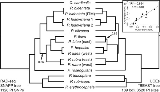
Species tree analyses of SNPs from the RAD-seq and UCE data sets in SNAPP (1128 and 605 SNPs, respectively) yielded identical results (Fig. 3) to those identified in the analyses of concatenated UCE data (Fig. 1). When limited to loci with a minimum of 10 PIS or 20 PIS, all UCE species tree methods identified the same relationships as the SNAPP analyses (Fig. 3, Table 3, Supplementary Information, available on Dryad). A strong correlation existed between branch lengths recovered in RAD-seq SNAPP and UCE *BEAST analyses (, ; Inset of Fig. 3). Although branch lengths were highly correlated, the RAD-seq tree had consistently shorter branch lengths than the UCE tree, particularly noticeable in terminal branches. Branch lengths may have been shorter in the RAD tree due to only using PIS, thereby reducing the amount of intraspecific and intraindividual genetic variation (i.e., autapomorphies). For both UCEs and RAD-seq data, SVDquartets analyses identified identical topologies to SNAPP and *BEAST analyses, with the exception of relationships within the Hepatic Tanager clade (P. hepatica P. lutea P. flava; Fig. 2). Varying minimum stack depth (RAD-seq data sets) changed the level of support for the two Hepatic Tanager clade topologies (Fig. 2) in SVDquartets analyses, but did not affect relationships among any other taxa (Supplementary Information, available on Dryad).
Identical species tree topologies from RAD-seq (SNAPP analysis) and UCE (*BEAST analysis) data sets. Most analyses, of both RAD-seq and UCE data, identified these relationships, with the exception of some analyses using gene trees with many uninformative UCE loci (Table 3). All unlabeled branches received greater than 0.95 posterior support values. The RAD-seq data set included only parsimony informative (PI; i.e., no singletons) sites. The UCE data set analyzed here included only highly informative loci (10 or more PI sites). The inset shows the comparison of relative branch lengths (BLs) between trees, with a slope () of approximately 0.8.
Summary of RAD-seq and UCE-data set phylogeny reconstruction methods used in this study.
 |
 |
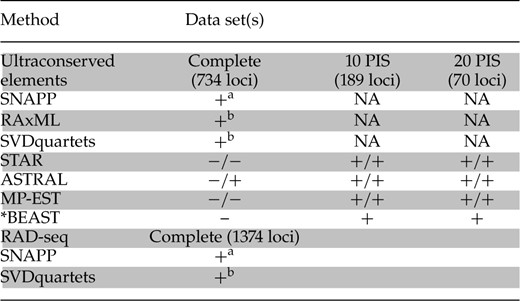
Notes: Species tree methods were used on three UCE data sets: (1) complete matrix [734 loci, 5052 PIS], (2) loci with a minimum of 10 PIS (189 loci, 3520 PIS), and (3) loci with a minimum of 20 PIS (70 loci, 1901 PIS). If the estimated phylogeny matched the hypothesized best tree [Fig. 3; excluding relationships within Hepatic Tanager clade (P. hepatica P. lutea P. flava)], it is marked with a (+). Conversely, an estimated phylogeny that did not match the best tree is marked with a (−). For STAR, ASTRAL, and MP-EST, the results are labeled for analyses using PhyML gene trees or RAxML gene trees on the left/right, respectively.
aSNAPP was run using a data set with only SNPs (1128 and 605 SNPs for the RAD-seq and UCE data sets, respectively).
bRAxML and SVDquartets were run on a concatenated data set with all loci, including variant and invariant sites.
Summary of RAD-seq and UCE-data set phylogeny reconstruction methods used in this study.
 |
 |
Notes: Species tree methods were used on three UCE data sets: (1) complete matrix [734 loci, 5052 PIS], (2) loci with a minimum of 10 PIS (189 loci, 3520 PIS), and (3) loci with a minimum of 20 PIS (70 loci, 1901 PIS). If the estimated phylogeny matched the hypothesized best tree [Fig. 3; excluding relationships within Hepatic Tanager clade (P. hepatica P. lutea P. flava)], it is marked with a (+). Conversely, an estimated phylogeny that did not match the best tree is marked with a (−). For STAR, ASTRAL, and MP-EST, the results are labeled for analyses using PhyML gene trees or RAxML gene trees on the left/right, respectively.
aSNAPP was run using a data set with only SNPs (1128 and 605 SNPs for the RAD-seq and UCE data sets, respectively).
bRAxML and SVDquartets were run on a concatenated data set with all loci, including variant and invariant sites.
The complete UCE matrix (734 loci) yielded three different topologies from different analyses. The ASTRAL method—using RAxML gene trees, but not PhyML gene trees—was the only analysis to produce concordant species trees between the complete data set and the data sets limited to highly informative loci. The ASTRAL analysis was also the only case in which the input gene trees (RAxML vs PhyML) had any impact on species tree topology (aside from the Hepatic Tanager clade). All other trees inferred from STAR, ASTRAL (PhyML only), and MP-EST with the full dataset were identical to one another. These analyses all identified P. ludoviciana as paraphyletic with P. bidentata monophyletic but nested within P. ludoviciana. The *BEAST analysis with the complete data set yielded the most disparate—but strongly supported—relationships within Piranga. Here, eight species and three clades contained different sister relationships (Supplementary Information, available on Dryad). Differences between the *BEAST tree and other analyses occurred in parts of the tree with short internodes (∼2% or less of total tree height). For example, Piranga leucoptera was found sister to Piranga erythrocephala rather than Piranga rubriceps (as in all other analyses). Additionally, P. rubra was not found to be sister to the Hepatic Tanager clade, but rather sister to a clade of P. bidentata, P. ludoviciana, P. olivacea, P. flava, P. hepatica, and P. lutea. These differences highlight the effect of uninformative UCE loci on species tree analyses (especially *BEAST; Table 3), especially in situations with short internode lengths.
Discussion
Here, we provide a comparison of RAD-seq and UCE data for phylogenetic inference using a suite of species tree inference methods. We fully resolved the phylogeny of Piranga and found nonmonophyly of P. lutea. However, we found that less informative UCE loci—and their respective gene trees—negatively impact some species tree methods. The bias caused by less informative loci is not likely to be restricted to UCE data sets, but biologists have generally not used gene trees for RAD-seq loci, likely due to limited information content per RAD locus. Indeed, analyses using SNPs extracted from UCE data—including all loci—recovered the hypothesized best topology, suggesting the negative impacts simply stem from using gene trees from many UCE loci with little information content.
Utility of RAD-seq and Target Capture for Phylogenetic Inference with Mixed Levels of Divergence
The utility of RAD-seq data for use in inferring interspecific phylogenies with deep divergences has been shown using in silico genome digests (e.g., Cariou et al. 2013) and empirical data (e.g., Cruaud et al. 2014). However, the nature of RAD-seq methodologies introduces genealogical biases in obtaining orthologous genetic markers (Arnold et al. 2013). Because the number of comparable RAD markers among species deteriorates through time because of mutations at restriction sites, estimating deep divergences using RAD-seq data may be problematic because cut sites preserved across deep phylogenies likely occur in regions that evolve at lower rates than other parts of the genome (Rubin et al. 2012). This potential bias raises the question: Can RAD-seq data adequately estimate a phylogeny across a moderately divergent taxonomic group? Here, we compared the ability of RAD-seq and UCE data to estimate a phylogeny in Piranga. We found that analysis of RAD-seq data identified a phylogenetic topology identical to that derived from UCE data (Fig. 3). This result suggests that the method of data collection (RAD-seq vs. UCEs) does not necessarily influence the results of species tree analyses at intermediate levels of divergence.
Two recent studies investigated the utility of RAD-seq and target capture for phylogenetic estimation at different timescales. In a shallow (<5 myr) phylogeographic study, Harvey et al. (2013) found concordant results between data sets. Conversely, in a deeper systematic study (15–55 myr), Leaché and colleagues (2015) found conflict between methods depending on how the data were analyzed. Using target capture data, Leaché et al. (2015) consistently found the same species tree, using both concatenation and coalescent-based methods. Conversely, when using RAD-seq data, no species trees matched that of the species tree from target capture data (Leaché et al. 2015). Additionally, using only the RAD-seq data, Leaché and colleagues (2015) identified different topologies between concatenation and species tree methods, as well as differences within a method (e.g., using only concatenation) when different clustering thresholds were used to group RAD loci.
We provide here a view at an intermediate timescale (0.5–6 myr), with denser sampling (multiple individuals per phylogenetic tip) that allowed a broader range of species tree inference methods (Table 3), and find concordant results among data sets (Fig. 3; Table 3). Unfortunately, our study system and design differed from Leaché et al. (2015) in multiple respects. First, we used a more recent timescale, which may have facilitated the use of both target-capture- and RAD-seq-based analyses. Second, different restrictions of coverage across loci (i.e., minimum depth of sequence reads), in both target capture and RAD-seq data sets, could potentially influence species tree inference. Finally, sampling different numbers of individuals per phylogenetic tip (i.e., population or species) could influence the power to resolve relationships.
Evolutionary History and Taxonomy
We identified a strongly supported phylogeny, which was mostly consistent with previous mtDNA phylogenies (Burns 1998, Shepherd and Burns 2007), with a few important differences. Most mtDNA phylogenies identified Piranga roseogularis as the sister taxon to all other Piranga; however, we find a clade of P. erythrocephala, P. leucoptera, and P. rubriceps as sister to all other Piranga. In addition, the positions of P. rubra and P. olivacea with respect to other Piranga were unclear in the mtDNA studies, but are clarified with our data. Piranga rubra is sister to the Hepatic Tanager clade (P. flava, P. hepatica, P. lutea), and P. olivacea is sister to a clade including P. bidentata and P. ludoviciana. A recent phylogenetic study of Emberizoidea, which includes Piranga and many other genera, identified many of the relationships we found (Barker et al. 2015). The only discrepancy between Barker and colleagues' (2015) phylogeny and ours was the position of P. olivacea within the clade containing P. olivacea, P. bidentata, P. ludoviciana, P. flava, P. lutea, P. hepatica, and P. rubra.
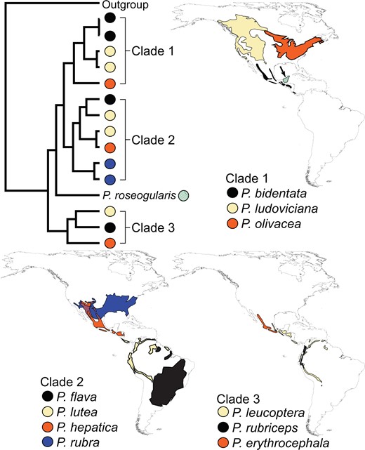
Comparison of three closely related lineages (as identified in Fig. 4) reveals that only one contains complete allopatric replacements. This pattern suggests that allopatric replacement is prevalent within Piranga during early divergence, soon followed by renewed sympatry. For example, P. hepatica, P. lutea, and P. flava are all allopatric replacements, with partial sympatry with sister species P. rubra. This pattern is repeated in clade 3 (Fig. 4); here, P. leucoptera and P. rubriceps are allopatric replacements of one another, with their sister species, P. erythrocephala, partially sympatric with both. These patterns suggest that early stages of differentiation are due to geographic separation, lending support to allopatric speciation as the main mechanism of diversification in Piranga.
Allopatric replacement in one of three main clades in Piranga. All distributions represent breeding range. Piranga roseogularis (diagonal stripes and indicated with an arrow, shown with Clade 1) is allopatric to all other species and present only in the Yucatan Peninsula of Mexico. Note that P. lutea (Clade 2) has a disjunct distribution, where an eastern individual is sister to P. flava, and a western individual is sister to P. hepatica. The only case of strict allopatric replacement within a clade is exhibited in Clade 1.
We found that one currently recognized species—P. lutea—is not monophyletic. A sample of P. lutea (subspecies haemelea) from the Guiana Shield is sister to P. flava, whereas a sample of western P. lutea (subspecies lutea) from the Andes is sister to P. hepatica. Although Burns (1998) did not find this relationship, their results do not contradict these relationships of P. lutea. Burns (1998) found western P. lutea sister to P. hepatica; however, the disjunct eastern range of P. lutea was not sampled in their study. These results may suggest that the Hepatic Tanager clade may be more than three distinct species because the Highland Tanager (P. lutea) has two distinct phylogenetic groups that are sister to different recognized species within the clade. The two lineages of P. lutea represent geographically and phenotypically differentiated subspecies of P. lutea (Hilty 2016); additionally, the other two taxa within the Hepatic Tanager group—P. flava and P. hepatica—show phenotypic differences from P. lutea (Hilty 2016). Differential morphologies, geographic ranges, and genetic histories lend support to each of the four lineages being considered distinct species under the evolutionary species concept (Wiley and Lieberman 1981), where all of the four taxa are on distinct evolutionary trajectories. Alternatively, these results could be interpreted as suggesting that the four groups of Hepatic Tanager are not each valid species, and that only one species exists. This alternative is plausible because the divergences within this clade are similar to those within other Piranga species with intraspecific sampling (Fig. 1) Additionally, the phenotypic differences between the taxa are complicated due to large seasonal and age plumage variation (Hilty 2016), for which we lacked solid geographical sampling because of the scope of this study. This clade warrants future phylogeographic investigation.
Import of Informative Loci for Species Tree Estimation
Although concatenated and SNP-based analyses of the overall UCE data set produced results concordant with methods using RAD-seq data, species tree analyses—those that utilize gene trees of each locus—that included low-information loci appeared to produce unreliable results (also see Hosner et al. 2016). Species-tree analyses of the complete UCE matrix (including uninformative loci) produced multiple distinct topologies; most species tree analyses recovered a slightly changed topology whereas the *BEAST analysis identified a much different topology. Conversely, species-tree analyses of data sets that included only informative loci (i.e., strong loci) produced the same species tree estimate for every method. Interestingly, longer loci generally had more PIS (Table 2), suggesting that researchers should strive to use library preparation methods that produce longer loci. Differences here are likely due to how different species tree methods handle gene trees from uninformative and low information loci. For example, our complete UCE matrix contained 129 loci with no PIS, and a total of 448 loci with 5 or fewer PIS. It is unlikely that these loci with few informative sites provide much phylogenetic signal for most relationships in the phylogeny. The methods used for species tree analysis with the RAD-seq data (SNAPP and SVDquartets) potentially circumvent information-content issues by considering each site to have an independent genealogy under the coalescent (Bryant et al. 2012; Chifman and Kubatko 2014) and not relying on underlying gene tree topologies for species tree estimation (such as in gene tree-based coalescent methods). As such, some studies have used SNP data extracted from UCEs to estimate species trees (e.g., this study and McCormack et al. 2016) to potentially circumvent information content issues of some loci. Using these two methods (i.e., SVDquartets and SNAPP) with SNPs extracted from UCE loci, we identified the phylogeny recovered from RAD-seq data and concatenated UCE data (Figs. 1 and 3). As such, incorporating less informative loci had no negative impact when analyzed in a concatenated data set, or in a method utilizing only SNPs (Table 3).
When testing the performance of MP-EST for species tree inference in a six-taxon simulation, Liu et al. (2015) found that increasing the number of low-information loci did not increase the probability of obtaining the correct species tree (e.g., >80 loci), whereas high-information loci produced the correct species tree 100% of the time with as few as 30 loci. Similarly, Lanier et al. (2014) identified that high- and low-variation loci yielded tremendous differences in accuracy of species-tree methods and recommended that quality, and not just quantity of loci be considered for phylogenetic studies. Here, we provide an empirical example of this situation, where our data set of 70 high-information UCE loci (with 20 PIS or more) was more consistent across species tree analyses—and obtained our hypothesized best species tree—compared with the much larger complete data set (734 UCE loci) which included many low-information UCE loci.
Conclusions
We created RAD-seq and UCE data sets to infer the phylogeny of the bird genus Piranga, with the following goals: 1) Assess the utility and comparability of RAD-seq and UCE for interspecific comparisons, 2) fully resolve taxonomic relationships in Piranga, and 3) assess the impacts of uninformative UCE loci on species tree reconstruction. We identified a fully resolved phylogeny of Piranga, with concordant topologies between RAD-seq and UCE data. We identified novel relationships in Piranga, relative to a previous study, and found that one currently recognized species (P. lutea) is not monophyletic. Finally, we found conflicting results from species tree analyses that included gene trees from uninformative UCE loci, with completely congruent results when limiting species tree analyses to data sets with only highly informative loci or only utilizing less informative loci with concatenation or methods meant for SNPs alone.
Data Accessibility
All raw sequence data are archived on the NCBI Sequence Read Archive under BioProject ID PRJNA296706. Scripts used in this project are in GitHub repositories (github.com/carloliveros, github.com/jdmanthey).
Author Contributions
All authors worked on conception of the project and completion of the manuscript. JDM and LCC performed laboratory work. JDM analyzed the data.
Supplementary Material
Data available from the Dryad Digital Repository: http://dx.doi.org/10.5061/dryad.j5n06.
Funding
This work was supported by a National Science Foundation (NSF) Doctoral Dissertation Improvement Grant [DEB-1406989 to JDM and RGM], a University of Kansas (KU) Graduate Research Grant [to JDM], a grant from the KU Research Investment Council [to RGM], a KU Biodiversity Institute Leamann Harris Award [to JDM and LCC], and NSF grants [to KJB (DEB-1354006) and RGM (DEB-1241181)].
Acknowledgments
The authors would like to thank the many institutions that provided tissue loans for this research: Field Museum of Natural History, Louisiana State University Museum of Natural Science, the Museo de Zoología de la Facultad de Ciencias at Universidad Nacional Autónoma de México, San Diego State University Museum of Biodiversity, and the University of Kansas Biodiversity Institute. They thank Carl Oliveros for helping them get set up with UCE laboratory preparation and analyses. They would like to thank KU Ornithology and members of the Phylogenomics Seminar for discussion of an early draft of the manuscript. The COBRE Genome Sequencing Core Laboratory, funded by National Institutes of Health (NIH) award number P20GM103638, provided laboratory facilities and services.
References
Author notes
Associate Editor: John McCormack



![RAxML topology of the concatenated UCE data (734 loci) for the Hepatic Tanager clade (from Fig. 1). At the tips are STRUCTURE results from RAD-seq data (complete matrix of 2960 SNPs) for two, three, and four inferred populations (proportion of color informs inferred probability of population ancestry). On the right are possible species tree topologies within this clade. Three analyses exhibited strong support for relationships in the most supported topology [*BEAST and ASTRAL (UCEs), and SNAPP (RAD-seq)]. SVDquartets (RAD-seq) was the only analysis to strongly support the alternative topology. All other analyses identified a polytomy (<75% bootstrap support) of P. hepatica, P. lutea (west), and P. flava + P. lutea (east).](https://oup.silverchair-cdn.com/oup/backfile/Content_public/Journal/sysbio/65/4/10.1093_sysbio_syw005/4/m_syw005f2.jpeg?Expires=1716388981&Signature=y1j1EvD4j12C1JCWxYPT1lW-y1JAm6gat78b6x1VQ4hfP8nvAbApB~rQLynG-wtsMyA0ypk6n1k9lngQZIbf1oNK-0wvJjoOK-qWowbpQpheyjBNnU~XktNEBoNvmL0B5VEPfen2ZaYFI6NIEw19~01k-vmEaUDQWb4rz4Gin5Z04SdIQrFPRZZNasiCfu~m6Pe3zeF97RI0nWQmQqKuBSYGt5PgUsLgZ91NZPjNgOjWPVDk1qqnZ~zCy-dSuoZM8mWB4BxmnAc3vxKcgyEXk5pNaBjIjg8oJNRYgqaeeEvz~ytLTQndHCreFP6KjGK~DUtJcoSOhtTHCOTadHlbhQ__&Key-Pair-Id=APKAIE5G5CRDK6RD3PGA)
